Model geometries

---

I will use this post to record some properties and calculations in the model surface \(M_K\) of constant curvature \(K\). I have used Chapter 2 of Thurston’s “The Geometry and Topology of 3-Manifolds” as a reference while writing this. It is recommended for readers to skip all the junk I have written below and directly read that chapter. I found Chapter 4.5 of Christian Bär’s lecture notes on differential geometry to be helpful while studying hyperbolic trigonometry, and I have tried to emulate the exposition at the end.

The model surface of constant curvature \(K\) is the sphere \(S^2_R\) of radius \(R = 1/\sqrt{K}\) if \(K > 0\), the Euclidean plane \(\Bbb R^2\) if \(K = 0\), and the hyperbolic plane \(\Bbb H^2_R\) of “imaginary radius” \(R = 1/\sqrt{-K}\) if \(K < 0\). We can define these spaces in a unified manner as follows: Let \(\epsilon_K\) denote the sign of \(K\), which is \(1\) if \(K > 0\), \(-1\) if \(K < 0\) and \(0\) if \(K = 0\). We shall equip the Euclidean space \(\Bbb R^3\) with the following bilinear form:

\[\displaystyle \langle \mathbf{x}, \mathbf{y} \rangle_K = \epsilon_K x_1 y_1 + x_2 y_2 + x_3 y_3\]

This is of course not an inner product space if \(K \leq 0\). Such a pair of vector space and simply a bilinear form is often called a quadratic space. The corresponding quadratic form will be denoted by \(Q_K(\mathbf{x}) = \epsilon_K x_1^2 + x_2^2 + x_3^2\); we can recover the bilinear form from the quadratic form using the polarization identity, so these really carry the same information about the quadratic space. Note that our quadratic space \((\Bbb R^3, \langle \cdot, \cdot \rangle_K)\) is the usual inner product space \(\Bbb R^3\) if \(K > 0\), a degenerate quadratic space \(\Bbb R \times \Bbb R^2\) degenerate along the first coordinate and usual Euclidean inner product space on the second coordinate if \(K = 0\) and the (1+2)-dimensional Minkowski spacetime \(\Bbb R^{1, 2}\) if \(K < 0\), where \(x_1\) is the timelike coordinate and \(x_2, x_3\) are the spacelike coordinates.

If \(K > 0\), we consider the sphere of radius \(R = 1/\sqrt{K}\) inside this quadratic space, given by

\[\displaystyle S_R(K) = \{\mathbf{x} \in \Bbb R^3 : Q_K(\mathbf{x}) = R^2\} = \{\mathbf{x} \in \Bbb R^3 : x_1^2 + x_2^2 + x_3^2 = 1/K\}\]

We equip the tangent spaces of \(S_R(K)\) with the metric \(\langle \cdot, \cdot \rangle_K\). Since in the case of \(K > 0\) the bilinear form is positive definite, this is indeed a Riemannian metric without further thought. The resulting space is the sphere \(S^2_R\) of radius \(R = 1/\sqrt{K}\).

If \(K < 0\), consider the sphere of radius \(R = i/\sqrt{-K}\)(!) inside the quadratic space. The difference in notation will be explained below.

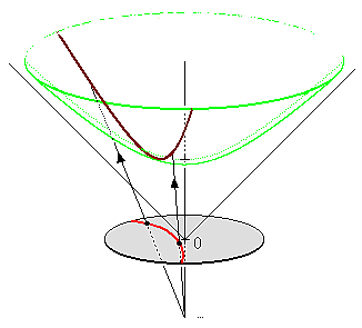
\[\displaystyle S^{\pm}_R(K) = \{\mathbf{x} \in \Bbb R^3 : Q_K(\mathbf{x}) = R^2\} = \{\mathbf{x} \in \Bbb R^3 : -x_1^2 + x_2^2 + x_3^2 = 1/K\}\]

In the Euclidean world, \(S^{\pm}_R(K)\) is a hyperboloid of two sheets in \(\Bbb R^3\). We consider the sheet \(S_R(K) = S^{\pm}_R(K) \cap \{x_1 > 0\}\) which lies in the “future” (interpreting \(x_1\) as the timelike coordinate) and equip the tangent spaces of \(S_R(K)\) with the bilinear form \(\langle \cdot, \cdot \rangle_K\). There is a precise way to talk about future and past in the Minkowski spacetime: the kernel of the bilinear form is given by

\[\{Q_K(\mathbf{x}) = 0\} = \{\mathbf{x} \in \Bbb R^3 : x_2^2 + x_3^2 = x_1^2\}\]

which is a cone in \(\Bbb R^3\). This is called the light cone, which consists of all the vectors in the direction of light emanating from the event \(\mathbf{0} = (0, 0, 0)\) in the space \(\{0\} \times \Bbb R^2\) at the time-slice \(x_1 = 0\). It was pointed out to me that the intuitive reason that the direction of light should be orthogonal to itself is because such directions are the only things which are coordinate-invariant (which, if there is any truth to the world, light trajectories must be); under any linear change of coordinates of spacetime, the light cone remains invariant. The future and past of the event \(\mathbf{0}\) is everything on and in the light cone, given by \(Q_K(\mathbf{x}) < 0\); intuitively this is because any point \(\mathbf{p}\) in the future or past of \(\mathbf{0}\) in the spacetime must be able to causally affect \(\mathbf{0}\), in the sense that, if it is in the past, one must be able to send a signal at most at the speed of light from \(\mathbf{p}\) that will reach \(\mathbf{0}\) eventually as time evolves in the positive direction, or if it is in the future, one must be able to send a signal at most at the speed of light from \(\mathbf{0}\) which will reach \(\mathbf{p}\) eventually, vice versa. Such trajectories must be trapped inside the light cone, essentially because their speed is bounded by the speed of light. Thus we declare future of \(\mathbf{0}\) to be anything in or on the positive half of the light cone and the past to be anything in or on the negative half of the light cone. It is worth mentioning on the side that vectors \(\mathbf{x}\) for which \(Q_K(\mathbf{x}) > 0\) are called spacelike, essentially because restricted to the space at time-slice \(x_0 = 0\), \(\langle \cdot, \cdot \rangle_K\) is the completely familiar Euclidean inner product, which is positive definite. Therefore whenever a vector has a spacelike coordinates dominating the timelike coordinate, the bilinear form will be positive definite on it, and thus it is called spacelike. The spacelike vectors consists of the exterior component of the light cone.

But this was a long digression. The point I wanted to make was that the hyperboloid \(S_R^{\pm}(K)\) is defined by the equation \(Q_K(\mathbf{x}) = R^2 = -1/K\), which is negative, therefore is contained in the light cone. The surface \(S_R(K)\) is the future half of this hyperboloid. Note that the restrictions of the bilinear form \(\langle \cdot, \cdot \rangle_K\) to the tangent spaces of \(S_R(K)\) are nondegenerate, since the tangent vectors to the future sheet of the hyperboloid are spacelike! It is possible to see this by observing that the light cone is asymptotic to the hyperboloid. Therefore in particular \(\langle \cdot, \cdot \rangle_K\) is positive definite on the tangent spaces of \(S_R(K)\), making it a Riemannian 2-manifold. It is possible to describe an isometry \(S_R(K) \to \Bbb H^2_R\) to the Poincare disk model by projecting \(S_R(K)\) to the disk \(\Bbb D_R \subset \{0\} \times \Bbb R^2\) of radius \(R = 1/\sqrt{-K}\), radially along lines through \((-1/\sqrt{-K}, 0, 0)\). A formula as such is

\[\displaystyle (x_1, x_2, x_3) \mapsto \left (\frac{x_2}{1 + \sqrt{1 - K(x_2^2+x_3^2)}}, \frac{x_3}{1+\sqrt{1 - K(x_2^2+x_3^2)}} \right )\]

Note how this is completely analogous to the the formula for the stereographic projection of \(S^2 \setminus \{\mathbf{N}\}\) to \(\Bbb R^2\). We shall chase the metric on \(S_R(K)\) to a metric on \(\Bbb D_R\) and show that it is indeed the Poincare metric. Let us write coordinates on \(\mathbb{R}^{1, 2}\) as \((t, \mathbf{x})\) for readability and suggestiveness, where \(t\) denotes the timelike coordinate and \(\mathbf{x} = (x_1, x_2)\) are the spacelike coordinates. We write the map above as \(\phi : S_R(K) \to \Bbb H^2\), \(\phi(t, \mathbf{x}) = \mathbf{x}/(1 + t \sqrt{-K})\). Then the Jacobian matrix of this map evaluated at \(p = (t, \mathbf{x})\) is given by

\[\displaystyle D\phi(p) = \begin{pmatrix} -x_1\sqrt{-K}/(1 + t\sqrt{-K})^2 & 1/(1+t\sqrt{-K}) & 0 \\ -x_2\sqrt{-K}/(1 + t\sqrt{-K})^2 & 0 & 1/(1 + t\sqrt{-K}) \end{pmatrix}\]

Let \(v = (s_1, \mathbf{v}), w = (s_2, \mathbf{w}) \in T_p S_R(K)\) be two tangent vectors on \(S_R(K)\) at \(p\). From the Jacobian formula, we see

\[\displaystyle \begin{aligned} D\phi(p)(v) &= - \sqrt{-K} \frac{s_1 \mathbf{x} }{(1 + t \sqrt{-K})^2} + \frac{\mathbf{v}}{1 + t\sqrt{-K}} \\ D\phi(p)(w) &= - \sqrt{-K} \frac{s_2 \mathbf{x}}{(1 + t\sqrt{-K})^2} + \frac{\mathbf{w}}{1 + t\sqrt{-K}} \end{aligned}\]

We can relate our bilinear form with the spacelike Euclidean dot product as:

\[\langle (t, \mathbf{a}), (s, \mathbf{b}) \rangle_K = - ts + \mathbf{a} \cdot \mathbf{b}\]

So using the fact that \(p = (t, \mathbf{x})\) is a norm \(i/\sqrt{-K}\) vector, and \(v, w\) are tangential to \(S_R(K)\) at \(p\), we obtain \(\mathbf{x} \cdot \mathbf{x} = t^2 + K^{-1}\), \(\mathbf{v} \cdot \mathbf{x} = s_1 t\) and \(\mathbf{w} \cdot \mathbf{x} = s_2 t\). With these identities in mind, we shall take the Euclidean dot product of the vectors \(D\phi(p)(v)\) and \(D\phi(p)(w)\) in \(\Bbb R^2\):

\[\displaystyle \begin{aligned}D\phi(p)(v) \cdot D\phi(p)(w) &= -K \frac{s_1 s_2 \mathbf{x} \cdot \mathbf{x}}{(1 + t\sqrt{-K})^4} - \sqrt{-K} \frac{s_1 \mathbf{x} \cdot \mathbf{w} + s_2 \mathbf{x} \cdot \mathbf{v}}{(1 + t\sqrt{-K})^3} + \frac{\mathbf{v} \cdot \mathbf{w}}{(1 + t\sqrt{-K})^2} \\ &= -K \frac{s_1 s_2 (t^2 + K^{-1}) }{(1 + t\sqrt{-K})^4} - \sqrt{-K} \frac{2 s_1 s_2 t}{(1 + t\sqrt{-K})^3} + \frac{\mathbf{v} \cdot \mathbf{w}}{(1 + t\sqrt{-K})^2} \\ &= \frac{-s_1 s_2 + \mathbf{v} \cdot \mathbf{w}}{(1 + t\sqrt{-K})^2} = \frac{\langle v, w \rangle_K}{(1 + t\sqrt{-K})^2}\end{aligned}\]

Now note that

\[\displaystyle \|\phi(p)\|^2 = \frac{\|\mathbf{x}\|^2}{(1 + \sqrt{-K} t)^2} = \frac{t^2 + K^{-1}}{(1 + t\sqrt{-K})^2} = -\frac{1}{K} \frac{t \sqrt{-K} - 1}{t \sqrt{-K} + 1}\]

So \(1 + K \|\phi(p)\|^2 = 2/(1 + t \sqrt{-K})\), and we therefore we can replace the factor of \((1 + t \sqrt{-K})^2\) appearing above by \(4/(1 + K\|\phi(p)\|)^2\). Putting it all together,

\[\displaystyle \langle v, w \rangle_K = 4 \frac{D\phi(p)(v) \cdot D\phi(p)(w)}{(1 + K\|\phi(p)\|)^2} = \phi^* \left ( 4 \frac{dx^2 + dy^2}{(1 + K(x^2 + y^2))^2} \right ) = \phi^* \omega_{P}\]

Where \(\omega_P\) is exactly the Poincare metric on \(\Bbb D_R\) in the disk model of \(\Bbb H^2_K\). It is worth noting that \(\omega_P\) is a pointwise multiple of the Euclidean metric on the disk, therefore hyperbolic angles drawn on the disk are the same as Euclidean angles, since scaling in the metric does not change measurements of angles. Such equivalences of metrics are called conformal equivalences; we just proved that the stereographic projection of the hyperboloid model to the disk is conformal, much like the stereographic projection of the sphere to the plane. In fact, if one computes the pullback of the spherical metric on \(S^2_K\) to \(\Bbb R^2\) under the stereographic projection, one would obtain a metric identical to \(\omega_P\) except with \(K\) positive (Compute it!). This implies for a flat creature who does not have access to the third dimension, spherical geometry is as unnatural as hyperbolic geometry!

The isometry group of the Riemannian manifold \(S_R(K)\) is the isotropy group \(O_K\) of the quadratic form \(Q_K\), consisting of all matrices in \(\mathrm{GL}_3(\Bbb R)\) preserving the bilinear form \(\langle \cdot, \cdot \rangle_K\), with a mild modification for \(K < 0\) to throw away the isometries which switch the two sheets of the hyperboloid \(S_R^{\pm}(K)\), i.e, only consider the causal orientation preserving isometries. In case of \(K > 0\), this is the orthogonal group \(O(3)\) and for \(K < 0\), this is the orthochronous Lorentz group \(O^+(1, 2)\). The spatial orientation preserving subgroup is denoted as \(SO(1, 2)\), and the elements of this group are Lorentz transformations of the (1+2)-dimensional spacetime. These are generated by spatial rotations, given by

\[\displaystyle R_\theta = \begin{pmatrix} 1 & 0 & 0 \\ 0 & \cos(\theta) & \sin(\theta) \\ 0 & -\sin(\theta) & \cos(\theta) \end{pmatrix}\]

and the so-called Lorentz boosts along various axis. For example, a Lorentz boost along the respective two spatial axes are given by

\[\displaystyle L^1_\zeta = \begin{pmatrix} \cosh(\zeta) & \sinh(\zeta) & 0 \\ \sinh(\zeta) & \cosh(\zeta) & 0 \\ 0 & 0 & 1 \end{pmatrix}, \;\;\; L^2_\zeta = \begin{pmatrix}\cosh(\zeta) & 0 & \sinh(\zeta) \\ 0 & 1 & 0 \\ \sinh(\zeta) & 0 & \cosh(\zeta) \end{pmatrix}\]

It can be easily checked that the isometry group of \(S_K(R)\) acts transitively on \(S_K(R)\), and the stabilizer subroup of a point is isomorphic to \(O(2)\) regardless of \(K\) (to see this in \(\Bbb H^2_K\), find a convenient point, eg, the vertex of the hyperboloid and observe that all the stabilizing elements are spatial rotations). This proves that the model geometries \(M_K\) are symmetric spaces: if \(K > 0\) it is \(O(3)/O(2)\), if \(K < 0\) it is \(O^+(1, 2)/O(2)\).

Let us try to understand the geodesics of \(\Bbb H^2_K\) using this information. For any 2-dimensional subspace \(H \subset \Bbb R^2\) such that \(H\) intersects the positive sheet of the hyperboloid \(S_R^{\pm}(K)\), the bilinear form \(\langle \cdot, \cdot \rangle_K\) restricts to a nondegenerate form on \(H\) that makes it a hyperbolic quadratic plane, as pictorially evident by seeing that the kernel of the restricted form is union of two lines in \(H\), obtained from intersecting \(H\) with the light cone. Choose an orthonormal basis \(\{v_1, v_2\}\) in \(H\) with respect to this form, and extend it to an orthonormal basis \(\{v_1, v_2, v_3\}\) of \(\Bbb R^{1, 2}\). Let \(A = (v_1, v_2, v_3)\); then \(A \in O^+(1, 2)\) such that \(A\mathbf{e}_i = v_i\) for \(1 \leq i \leq 3\). Therefore \(A\) takes the span of \(\mathbf{e}_1, \mathbf{e}_2\), i.e., the plane \(x_3 = 0\) to the plane \(H\). Observe that the the matrix \(B = \mathrm{diag}(1, 1, -1)\) is an element of \(O^+(1, 2)\) which reflects along the plane \(x_3 = 0\); the timelike direction is not affected in this process so it is safely an orthochronous Lorentz transformation. Finally consider the element \(ABA^{-1} \in O^+(1, 2)\), and observe that this fixes \(H\) since \(B\) fixes \(x_3 = 0\). Thus, \(ABA^{-1}\) is an isometric involution of \(S_R(K)\) fixing the curve \(H \cap S_R(K)\). Hence, it must be a geodesic of \(S_R(K)\). Moreover these are all the geodesics of \(S_R(K)\), since through any point with a given tangent vector, one can draw a 2-dimensional section of the hyperboloid passing through that point, tangential to the vector. This is analogous to the situation for \(K > 0\) where the geodesics on the sphere \(S^2_R\) are given by slicing it by a plane through the origin, which traces out a great circle on the sphere.

We can write down explicit formulas for geodesics on \(S_R(K)\). Namely, if \(\gamma : \Bbb R \to S_R(K)\) is an arclength parametrized geodesic passing through \(\gamma(0) = (1/\sqrt{-K}, 0, 0)\), it must be of the form

\[\displaystyle \gamma(t) = \frac{1}{\sqrt{-K}} \left ( \cosh(t \sqrt{-K}), \sinh(t \sqrt{-K}) \cos(\theta), \sinh(t \sqrt{-K}) \sin(\theta) \right )\]

To see this, observe \(\langle \gamma, \gamma \rangle_K = R^2\), so \(\gamma\) lies on \(S_R(K)\), and \(\langle \gamma', \gamma' \rangle_K = 1\) which implies \(\gamma\) is arclength parametrized. \(\gamma\) clearly lies on the plane spanned by \((1/\sqrt{-K}, 0, 0)\) and \((0, \cos(\theta), \sin(\theta))\), so it must be a geodesic, as required. Note the similarity with formulas for arclength parametrized geodesics on \(S_R(K) \cong S^2_R\) for \(K > 0\) passing through \((1/\sqrt{K}, 0, 0)\), which can be written down by simply replacing the hyperbolic trigonometric functions with usual trigonometric functions:

\[\displaystyle \gamma(t) = \frac{1}{\sqrt{K}} \left ( \cos(t \sqrt{K}), \sin(t \sqrt{K}) \cos(\theta), \sin(t \sqrt{K}) \sin(\theta) \right )\]

This describes the geodesics of \(\Bbb H_K^2\) in the hyperboloid model completely. If we project to the unit disk conformally, we obtain that the geodesics in the disk model are exactly diameters as well as semicircular arcs which hit the boundary circle perpendicularly, as illustrated in the following picture:

Here on the left we have an illustration of a geodesic tessellation of \(\Bbb H_K^2\) in Poincare disk model, and on the right is “Circle Limit III” by Escher, who mistakenly thought that the white lines are geodesics, but in fact they meet the boundary circle in somewhere close to 80 degrees, as Coxeter found out:

Earlier we found that if \(M\) is a Riemannian 2-manifold of constant Gaussian curvature \(K\), then for any geodesic \(\gamma : [0, c] \to M\) with initial point \(\gamma(0) = p\) and a normal Jacobi field \(J\) along \(\gamma\), its length \(f(t) = \|J(t)\|\) must satisfy the second order linear differential equation \(f'' + K f = 0\). Solving with initial conditions \(J(0) = 0\) and \(J'(0) = \mathbf{e}_p\) we obtain

\[\displaystyle \begin{aligned} J(t) &= \frac{\sin(t \sqrt{K})}{\sqrt{K}} \mathbf{e} \;\; \text{if} \;\; K > 0 \\ J(t) &= t \mathbf{e} \;\; \text{if} \;\; K = 0 \\ J(t) &= \frac{\sinh(t \sqrt{-K})}{\sqrt{-K}} \mathbf{e} \;\; \text{if} \;\; K < 0\end{aligned}\]

Thus, in positive curvature, nearby geodesics starting at a common point “tend to” behave periodically, by diverging off, then coming back and converging to a point, and so forth. Similarly, in negative curvature, nearby geodesics starting at a common point “tend to” diverge from each other at an exponential rate. In zero curvature, nearby geodesics starting at a common point “tend to” grow linearly far apart. But the Jacobi field computation can only tell us about these tendencies as such; whether or not these actually happen is unclear. We shall show by some spherical and hyperbolic trigonometry that these do in fact happen in case of the model surface \(M_K\) of constant curvature \(K\).

Suppose we have a geodesic triangle \(\Delta = [P,Q,R]\) in \(M_K\) with vertices \(P, Q, R\), geodesic \(PQ, PR, QR\) of length \(a, b, c\) and angles opposite to the sides \(\alpha, \beta, \gamma\) respectively. For \(K = 0\), we have a convenient formula for \(c\) in terms of \(a, b\) and \(\gamma\), obtained using familiar trigonomentry, \(c^2 = a^2 + b^2 + 2ab\cos(\gamma)\). Imagine changing the triangle \(\Delta\) by fixing the vertex \(P\), but varying the sides \(a, b\) and the angle \(\gamma\). The formula gives an understanding on the change in \(c\) that comes from such maneuvers. Importantly, if \(a = b = T\), then \(c\) is proportional to \(T\), with the proportionality constant depending on the angle \(\gamma\) between the sides. This implies that in the flat plane, two geodesics starting at a point and run until time \(T\) will be a constant multiple of \(T\) apart. We would like to do similar calculations for \(K \neq 0\), but we would need to develop a theory of trigonometry in non-planar geometries to accomplish this, which we do in the next paragraph.

Motivated from the mysterious apparitions in earlier computations, define trigonometric functions in the model geometry of constant curvature \(K \neq 0\) by

\[\displaystyle \begin{gather*} \sin_K(x) = \frac{\sin(x\sqrt{K})}{\sqrt{K}} \;\; \text{if} \; K > 0 \;\; \text{and} \;\; \frac{\sinh(x \sqrt{-K})}{\sqrt{-K}} \;\; \text{if} \;\; K < 0 \\ \cos_K(x) = \frac{\cos(x\sqrt{K})}{\sqrt{K}} \;\; \text{if} \;\; K > 0 \;\; \text{and} \;\; \frac{\cosh(x \sqrt{-K})}{\sqrt{-K}} \;\; \text{if} \;\; K < 0\end{gather*}\]

Observe the trigonometric identity \(\cos_K^2(x) + \epsilon_K \sin_K^2(x) = 1/\vert K\vert\). In the earlier setup of the triangle \(\Delta = [P, Q, R]\) in \(M_K\), we can arrange \(P = (1/\sqrt{\vert K \vert}, 0, 0)\) by applying an isometry, and moreover we can do a (spatial, in case of \(K < 0\)) rotation so that \(Q\) is in the \(xy\)-plane. Then the whole geodesic \(PQ\) must lie in the \(xy\)-plane, implying \(Q = (\cos_K(a), \sin_K(a), 0)\). Define

\[\displaystyle \mathbf{M} = \begin{pmatrix} \sqrt{\vert K \vert} \cos_K(a) & \epsilon_K \sqrt{|K|} \sin_K(a) & 0 \\ \sqrt{|K|} \sin_K(a) & - \sqrt{|K|} \cos_K(a) & 0 \\ 0 & 0 & 1 \end{pmatrix}\]

\(\mathbf{M}\) is an orthogonal transformation if \(K > 0\) and composition of a Lorentz boost with a reflection along the \(xz\)-plane if \(K < 0\). Then we obtain a new geodesic triangle \(\mathbf{M} (\Delta) = [\mathbf{M}P, \mathbf{M}Q, \mathbf{M}R]\); but observe that \(\mathbf{M} P = Q\) and \(\mathbf{M} Q = P\). Let \(R' = \mathbf{M} R\)

Since \(PR\) makes an angle of \(\gamma\) with \(PQ\) in \(\Delta\), the plane that cuts out \(PR\) from \(M_K\) must make an angle of \(\gamma\) with the \(xz\)-plane. Therefore \(R = (\cos_K(b), \sin_K(b) \cos(\gamma), \sin_K(b) \sin(\gamma))\). On the other hand, \(PR'\) makes the same angle with \(PQ\) in \(\mathbf{M}(\Delta)\) as \(QR\) and \(QP\) in \(\Delta\), which is \(\beta\). Thus, \(R' = (\cos_K(c), \sin_K(c) \cos(\beta), \sin_K(c) \sin(\beta))\). Writing \(\mathbf{M} R = R'\) in coordinates,

\[\displaystyle \begin{pmatrix} \sqrt{|K|} \cos_K(a) & \epsilon_K \sqrt{|K|} \sin_K(a) & 0 \\ \sqrt{|K|} \sin_K(a) & - \sqrt{|K|} \cos_K(a) & 0 \\ 0 & 0 & 1\end{pmatrix} \begin{pmatrix} \cos_K(b) \\ \sin_K(b) \cos(\gamma) \\ \sin_K(b) \sin(\gamma) \end{pmatrix} = \begin{pmatrix}\cos_K(c) \\ \cos_K(c) \sin(\beta) \\ \sin_K(c) \sin(\beta)\end{pmatrix}\]

Computing out the identity obtained from the first entry, we get:

\[\displaystyle \cos_K(c) = \sqrt{|K|} \cos_K(a) \cos_K(b) + \epsilon_K \sqrt{|K|} \sin_K(a) \sin_K(b) \cos(\gamma)\]

This is the cosine formula for sides of a triangle. Written explicitly,

\[\displaystyle \begin{aligned}\cos(c\sqrt{K}) &= \cos(a\sqrt{K}) \cos(b\sqrt{K}) + \sin(a\sqrt{K}) \sin(b\sqrt{K}) \cos(\gamma) \;\; \text{if} \;\; K > 0 \\ \cosh(c\sqrt{-K}) &= \cosh(a\sqrt{-K}) \cosh(b\sqrt{-K}) - \sinh(a\sqrt{-K}) \sinh(b\sqrt{-K}) \cos(\gamma) \;\; \text{if} \;\; K < 0\end{aligned}\]

Set \(a = b = T\) and \(\gamma\) be constant. We get

\[\begin{aligned}\cos(c \sqrt{K}) &= 1 - \sin^2(T \sqrt{K}) (1 - \cos \gamma) \;\; \text{if} \;\; K > 0 \\ \cosh(c\sqrt{-K}) &= 1 + \sinh^2(T\sqrt{-K})(1 - \cos \gamma) \;\; \text{if}\;\; K < 0\end{aligned}\]

We inspect the cases \(K = 1\) (red curve) and \(K = -1\) (blue curve) in this Desmos snippet. Use the slider to change the value of \(0 \leq \gamma \leq \pi\). We see the value of \(c\) behaves periodically with respect to time \(T\) if curvature is positive, and exponentially grows with respect to time \(T\) if curvature is negative. This is the desired global result that we wanted to see.

I shall stop here for now but I might keep adding new stuff as I stumble across them later on. I’ll make a note of them whenever I do. Up next, more Jacobi fields.