Hilbert’s theorem and curiosities

---

The contents of this post emerged in the process of preparing and presenting a mini-course titled “Curvature: Geometry, Topology and Combinatorics” in an online math camp for high school students called Monsoon Math Camp. I acknowledge the community and in particular the students for prompting me to think about these questions.

It is a classical theorem of Hilbert that there is no smooth isometric immersion of the hyperbolic plane \(\Bbb H^2\) in \(\Bbb R^3\). I will begin with a proof of this fact, as outlined in do Carmo, “Differential Geometry of Curves and Surfaces”.

Suppose \(M \subset \Bbb R^3\) is an everywhere negatively curved surface. Then for any point \(x \in M\), \(M\) must “look like” a saddle around \(x\), with \(x\) being the saddle point, so one would imagine \(T_x M\) intersects \(M\) in a pair of lines, as in a saddle. These lines are called the asymptotic directions of \(M\) at \(x\). More precisely, observe that if \(\Bbb{II}\) is the second fundamental form on \(M\), \(\Bbb{II}_x\) is a nondegenerate indefinite symmetric bilinear form on \(T_x M\) since if \(v, w \in T_x M\) is a pair of principal directions, \(\Bbb{II}_x(v, v) > 0\) and \(\Bbb{II}_x(w, w) < 0\). Thus \(\Bbb{II}_x\) has nontrivial kernel on \(T_x M\), which is a 1-dimensional cone, i.e., a pair of lines on \(T_x M\). The pair of lines vary continuously with \(x\), so we can choose a local parametrization

\[\begin{align*}\mathbf{x} : U \subset \Bbb R^2 &\to M \\ (u, v) &\mapsto \mathbf{x}(u, v) \end{align*}\]

such that \(\mathbf{x}_u\) and \(\mathbf{x}_v\) are the asymptotic directions throughout the local patch \(\mathbf{x}(U) \subset M\), i.e., \(\Bbb{II}(\mathbf{x}_u, \mathbf{x}_u) = \Bbb{II}(\mathbf{x}_v, \mathbf{x}_v) = 0\). Denote the metric and the second fundamental form with respect to these coordinates as

\[\begin{align*}ds^2 &= E du^2 + 2F du dv + G dv^2 \\ \Bbb{II} &= e du^2 + 2f du dv + g dv^2, \end{align*}\]

as is convention. Note that \(e = f = 0\) since the coordinate directions are asymptotic.

Suppose moreover that \(M\) is constant curvature \(K < 0\). Then the surface normal \(\mathbf{n}\) is parallel to \(\mathbf{x}_{uv}\) throughout \(\mathbf{x}(U) \subset M\). This can be seen by the following sequence of computations: By definition of Gaussian curvature, \(\mathbf{n}_u \times \mathbf{n}_v = K \mathbf{x}_u \times \mathbf{x}_v\). We write the area element as \(A = \|\mathbf{x}_u \times \mathbf{x}_v\|\), so that \(\mathbf{x}_u \times \mathbf{x}_v = A \mathbf{n}\). Noting the identity \((\mathbf{n} \times \mathbf{n}_v)_u - (\mathbf{n} \times \mathbf{n}_u)_v = 2 \mathbf{n}_u \times \mathbf{n}_v\) we proceed to calculate:

\[\displaystyle \begin{aligned} \mathbf{n} \times \mathbf{n}_u = \frac1{A} (\mathbf{x}_u \times \mathbf{x}_v) \times \mathbf{n}_u &= \frac1{A} \left ( (\mathbf{x}_u \cdot \mathbf{n}_u) \mathbf{x}_v - (\mathbf{x}_v \cdot \mathbf{n}_u) \mathbf{x}_u \right ) \\& = \frac1{A} (e \mathbf{x}_v - f \mathbf{x}_u) = -\frac{f}{A} \mathbf{x}_u \end{aligned}\] \[\displaystyle \begin{aligned} \mathbf{n} \times \mathbf{n}_v = \frac1{A} (\mathbf{x}_u \times \mathbf{x}_v) \times \mathbf{n}_v &= \frac1{A} \left ( (\mathbf{x}_u \cdot \mathbf{n}_v) \mathbf{x}_v - (\mathbf{x}_v \cdot \mathbf{n}_v) \mathbf{x}_u \right ) \\& = \frac1{A} (f \mathbf{x}_v - g \mathbf{x}_u) = \frac{f}{A} \mathbf{x}_v \end{aligned}\]

We know \(K = \det{\Bbb{II}}/A^2 = -f^2/A^2\), so that \(f/A = \sqrt{-K}\). Plugging everything in, we get \(\displaystyle 2\sqrt{-K} \mathbf{x}_{uv} = 2\mathbf{n}_u \times \mathbf{n}_v = 2K A \mathbf{n}\) which shows \(\mathbf{n} \parallel \mathbf{x}_{uv}\) as desired.

From the above we obtain \(E_v = 2\mathbf{x}_{uv} \cdot \mathbf{x}_u = 0\) and \(G_u = 2\mathbf{x}_{uv} \cdot \mathbf{x}_v = 0\). Thus, \(E = E(u)\) is a pure function of \(u\) and \(G = G(v)\) is a pure function of \(v\) respectively, and we can thus reparametrize the coordinates \(u, v\) separately so that \(E = 1\) and \(G = 1\), i.e., the coordinate curves are arclength parametrized. Thus in particular the rectangles formed by the coordinate curves \(\mathbf{x}(I) \subset M\), where \(I = [s_1, s_2] \times [t_1, t_2] \subset U\), be geometric parallelograms, i.e., have opposite sides of equal lengths. Moreover, \(F = \mathbf{x}_u \cdot \mathbf{x}_v = \cos(\theta)\) where \(\theta \in (0, \pi)\) is the angle between the coordinate directions. Thus the metric on the surface is:

\[ds^2 = du^2 + 2\cos(\theta) dudv + dv^2\]

We change coordinates by \(u = x + y\) and \(v = x - y\) to diagonalize the metric as

\[ds^2 = 4 \cos^2(\theta/2) dx^2 + 4 \sin^2(\theta/2) dy^2\]

For diagonalized metrics it is easy to compute curvature using the Gauss-Codazzi equations:

\[\displaystyle K = -\frac{1}{2\sqrt{EG}} \left ( \left ( \frac{E_y}{\sqrt{EG}} \right )_y + \left ( \frac{G_x}{\sqrt{EG}} \right )_x \right )\]

Plugging \(E_y = -2\sin(\theta)\theta_y\), \(G_x = 2\sin(\theta)\theta_x\) and \(\sqrt{EG} = 2\sin(\theta)\) in above, we get

\[\displaystyle K = -\frac{\theta_{xx} - \theta_{yy}}{4\sin(\theta)} = -\frac{\theta_{uv}}{\sin(\theta)}\]

So this special coordinate patch \(\mathbf{x} : U \to \mathbf{x}(U) \subset M\) on the constant negative curvature surface \(M\), known in literature as a Tchebyshef net, can be imagined as a fishnet pattern over the surface made by two sets of arclength parametrized coordinate curves, where each individual cell is a geometric parallelogram with internal angle \(\theta\) varying cellwise according to the partial differential equation

\[\theta_{uv} + K \sin(\theta) = 0\]

Intuitively, (I think) the formula for the curvature can be justified as follows: \(K\) is equal to the limit of the holonomy angle when parallel transporting over a loop divided by area bounded by the loop, as the loop shrinks to the constant loop. We start with a node of the Tchebyshef net, and an asymptotic direction, and parallel transport it over a cell of area \(\sin(\theta) st\) in the fishnet. The asymptotic curves in the saddle are geodesics as they are straightlines, and since \(M\) locally looks like the saddle we can assume upto first order that the asymptotic curves are geodesics. Then the holonomy upon parallel translating over the coordinate cube is \(-\theta_{uv} s t\) upto second order, hence in the limit \(K = -\theta_{uv}/\sin(\theta)\), as we computed.

Assume now that \(M\) is complete, and extend this to a global parametrization \(\mathbf{x} : \Bbb R^2 \dashrightarrow M\) by setting \(\mathbf{x}(0, 0) = p\) and defining \(\mathbf{x}(s, t)\) to be the point reached by running along the first coordinate asymptotic curve for time \(s\) and then the second coordinate asymptotic curve for time \(t\). Let the domain of the parametrization be \(E = \{(s, t) \in \Bbb R^2 : \mathbf{x}(s, t) \text{ is well-defined}\}\). If \((s_0, t_0) \in E\) we can lay a Tchebyshef net at \(\mathbf{x}(s_0, t_0)\) which would match \(\mathbf{x}\) in the intersection of the domain of definition, essentially by uniqueness of solutions to ODEs. Thus \(\mathbf{x}\) would be defined in a neighborhood of \((s_0, t_0)\) as well, hence \((s_0, t_0) \in E\) is an interior point. If \((s_\infty, t_\infty) \in E\) is a limit point, we can take a sequence \(\{(s_n, t_n)\}\) in \(E\) converging to \((s_\infty, t_\infty)\), so that \(q_n = \mathbf{x}(s_n, t_n)\) is a Cauchy sequence on \(M\) since coordinate distances are Euclidean by arclength parametrization of the coordinate curves; hence by metric completeness of \(M\) converges to some point \(q\) and we define \(\mathbf{x}(s_\infty, t_\infty) = q\). Thus, \((s_\infty, t_\infty) \in E\). These show that \(E \subset \Bbb R^2\) is a nonempty clopen subset, hence \(E = \Bbb R^2\) and thus \(\mathbf{x}\) is globally well-defined. It is clear that \(\mathbf{x}\) is a local diffeomorphism, since \(\mathbf{x}_u\) and \(\mathbf{x}_v\) are the two independent coordinate directions at every point.

Let \(\Omega \subset M\) be the image of \(\mathbf{x}\), which must be an open subset as \(\mathbf{x} : \Bbb R^2 \to M\) is a local diffeomorphism. Choose a point \(p \in \partial \Omega\) and lay a Tchebyshef net around \(p\). This will intersect \(\Omega\) and thus we shall find a point \(q \in \Omega\) whose asymptotic curve intersects that of \(p\), which is impossible since asymptotic curves emanating from \(\Omega\) stays inside \(\Omega\). Thus \(\Omega = M\) and \(\mathbf{x}\) is therefore surjective. It’s a little more fidgety to argue \(M\) is simply connected, \(\mathbf{x}\) is injective: do Carmo gives a fidgety argument for this, but let me attempt at a cleaner approach. The fiberwise nondegenerate symmetric indefinite billinear form \(\Bbb{II}\) reduced the structure group of the tangent bundle \(TM\) to \(O(1, 1)\). Therefore we have a corresponding classifying map \(M \to BO(1, 1)\); but since \(\pi_1(M) = 0\), this map lifts to the universal cover \(\widetilde{BO(1, 1)} = BSO^+(1, 1)\). This implies we can upgrade the “cone field” on \(M\) given by \(\ker \Bbb{II}\) to a pair of well-defined global null vector fields \(X, Y\) on \(M\). Since \(\mathbf{x}_u = X\) and \(\mathbf{x}_v = Y\), we obtain by existence and uniqueness of ODEs that two independent family of strands of the fishnet given by \(\mathbf{x}\) do not self-intersect, and every pair of independent strands intersect at a unique point. This therefore implies \(\mathbf{x}\) is injective. We needed simple connectedness of \(M\) crucially in the argument, because in general it is possible that an asymptotic curve intersects itself in a general surface of negative curvature immersed in \(\Bbb R^3\).

As a small detour at this point, observe that a Tchebyshef net is completely determined by the data of the fishnet angles, \(\theta : \Omega \subset \Bbb R^2 \to \Bbb R\) satisfying the PDE \(\theta_{uv} = - K \sin(\theta)\) relative to the geometric restriction \(0 < \theta < \pi\). This PDE is known as the sine-Gordon equation, and Hilbert’s theorem is the statement that there are no regular global solutions to this equation with the restriction \(0 < \theta < \pi\). The name derives from the fact that if we write the equation in space-time coordinates \(x = u + v\), \(t = u - v\) it transforms into \(\square \theta - K \sin(\theta) = 0\) where \(\square \theta = \theta_{tt} - \theta_{xx}\) is the d’Alembert operator with speed of light assumed to be \(1\), which in the low-amplitude case has first order approximation to a linear wave equation-type PDE \((\square - K)\theta = 0\) known as the Klein-Gordon equation. This is of course all reminiscent of 1-dimensional story with the simple harmonic oscillator, although I am not sure of what the precise physical meaning of this is. The sine-Gordon equation belongs to a class of nonlinear PDEs arising from physics known as soliton equations whose solutions are solitary waves \(u(x, t) = f(x - ct)\) with \(f\) rapidly decaying at infinity, which are called the soliton solutions and there exists a nonlinear superposition law of waves which gives rise to solutions asymptotic to sum of solitary waves \(\sum_{i = 1}^n f_i(x - c_i t)\) as \(t \to -\infty\) and \(\sum_{i = 1}^n f_i(x - c_i t + \phi_i)\) as \(t \to \infty\), which is to be interpreted as \(n\) solitary waves coming togather, interacting in a nonlinear fashion in a compact interval of time, and then dissipating off to infinity with no change in shape or velocities but individual phase shifts \(\phi_i\). Let us try to exhibit this phenomenon for the sine-Gordon equations in space-time coordinates with curvature \(K = -1\): plug \(\theta(x, t) = f(x - ct)\) as the soliton ansatz in \(\square \theta + \sin(\theta) = 0\) to obtain the ODE \((1 - c^2) f'' = \sin(f)\) where the rapid decay condition of the soliton is to be interpreted as \(\vert f(u)\vert, \vert f'(u)\vert \to 0\) as \(u \to \pm \infty\). Using this, we solve \(f(u) = 4 \arctan \exp(\pm \gamma (u - \phi))\) where \(\phi\) is the “phase” of the soliton and \(\gamma = 1/\sqrt{1 - c^2}\) is the “Lorentz factor” of the soliton with velocity \(c\). The solution with the positive sign in the argument is called a kink and the one with the negative sign is called an antikink. The 1-parameter surfaces of constant curvature \(-1\) corresponding to these solutions is the Dini family of pseudospheres

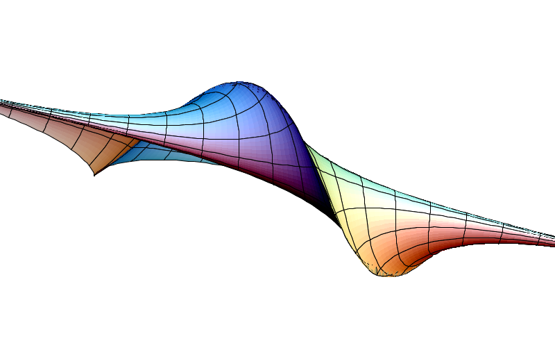
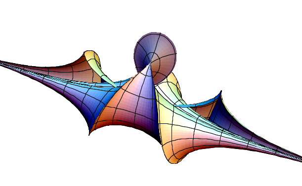
I used 3D-XplorMath to plot this image, and I really recommend downloading it and try to play with pseudospherical surfaces there. There is an animation option which can be used to see the family of surfaces as \(c\) varies. One can observe the “hump” along the curve of singularities on the surface to be propagating like a wave along the axis of the pseudospheres, reminiscent of a corkscrew. At some intermediate stage, the curve of singularities limit from a spiral to a circle, and at that moment the Dini surface is the plain vanilla pseudosphere that we all know and adore. I wanted to talk a bit more about how one obtains multisoliton solutions to the sine-Gordon equation using Bäcklund transforms but I realize I don’t understand it adequately enough myself to explain it in a concise manner. Instead, I will refer the reader to the excellent exposition “Geometry of Solitons” by Terng and Uhlenbeck for further information on soliton equations and how sine-Gordon is an example of such. Here is a picture of a surface of constant curvature -1 obtained from a 2-soliton formed by colliding a kink and an anti-kink:

We now proceed to prove Hilbert’s theorem. Suppose \(M \subset \Bbb R^3\) is a smoothly isometrically immersed copy of \(\Bbb H^2\), so by above we obtain a global Tchebyshef net \(\mathbf{x} : \Bbb R^2 \to M\) which is a bijective local diffeomorphism, hence a diffeomorphism as \(M\) is simply connected, and since \(K \equiv -1\), we have \(\theta_{uv} = \sin(\theta)\). Choose any coordinate rectangle \(I = [s_1, t_1] \times [s_2, t_2] \subset \Bbb R^2\). Then the area of \(\mathbf{x}(I) \subset M\) can be computed as:

\[\displaystyle \begin{aligned} \int_I A du dv &= \int_I \sin(\theta) du dv = \int_I \theta_{uv} du dv \\ & = \theta_{11} - \theta_{12} + \theta_{22} - \theta_{21} \\ &= (\alpha_{11} + \alpha_{12} + \alpha_{21} + \alpha_{22}) - 2\pi < 2\pi \end{aligned}\]

Where \(\theta_{ij}\) are the fishnet angles and \(\alpha_{ij}\) are the interior angles at the vertices \(\mathbf{x}(s_i, t_j)\) of the geometric rectangle \(\mathbf{x}(I)\), where the last inequality is just a consequence of the fact that \(\alpha_{ij} < \pi\). Taking the rectangles \(I = [-n, n]^2\) and letting \(n \to \infty\) shows that \(M\) has finite volume, bounded by \(2\pi\), which is a contradiction since \(\Bbb H^2\) is an infinite volume Riemannian surface. This also proves nonimmersability of any complete constant negative curvature surface in \(\Bbb R^3\), since we can compose the immersion with the exponential map \(\exp_p : T_p M \to M\) to get an immersion of \(T_p M\) with a metric of constant negative curvature \(K < 0\), and the metric can be scaled so that \(K \equiv -1\), in which case by Cartan’s theorem (known as Minding’s theorem for surfaces) \(T_p M\) is isometric to \(\Bbb H^2\), reducing it to Hilbert’s theorem.

As a remark, observe that throughout we did not quite require smoothness of the immersion since to do these curvature arguments we just need \(C^2\)-regularity. Thus, Hilbert’s theorem in fact proves there is no \(C^2\)-regular immersion of \(\Bbb H^2\) in \(\Bbb R^3\). There are however many such \(C^1\)-regular embeddings. To construct one we shall use the Nash-Kuiper \(h\)-principle. Call a smooth map \(f : (M, g) \to (N, h)\) of Riemannian manifolds a short map if \(f^* g < h\) in the sense of quadratic forms, i.e, \(\|f_* v\|_h < \|v\|_g\) for any \(v \in TM\).

Theorem (Nash-Kuiper): Let \((M^m, g)\) be a Riemannian manifold, and \(g_{\mathrm{Euc}}\) be the Euclidean metric on \(\Bbb R^n\) where \(m < n\). For any short immersion \(f : M \to \Bbb R^n\) and any \(\varepsilon > 0\) there exists \(C^1\)-regular isometric immersion \(f_1 : M \to \Bbb R^n\) such that \(\|f_1 - f\|_{C^0} < \varepsilon\), and \(f_1\) can be chosen to be an embedding if \(f\) is an embedding.

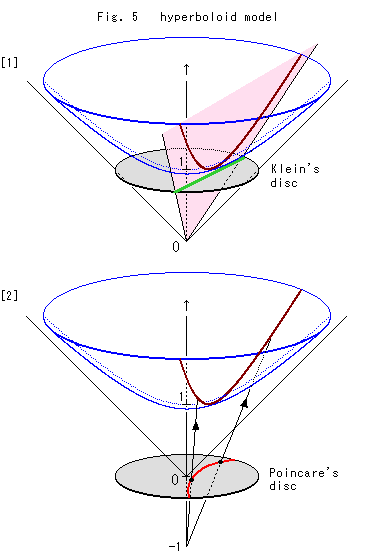
One model for the hyperbolic plane is the Beltrami-Klein disk model, which is the unit disk \(\Bbb D \subset \Bbb R^2\) equipped with the metric

\[\displaystyle ds^2 = \frac{dx^2 + dy^2}{1 - x^2 - y^2} + \frac{(xdx + ydy)^2}{(1 - x^2 - y^2)^2}\]

This can be obtained from the hyperboloid model discussed in the previous post, by stereographically projecting to a disk tangent to the vertex of the hyperboloid as opposed to an equatorial disk as in the Poincare disk model.

Then the canonical inclusion \(\Bbb D \to \Bbb R^3\) is a short embedding, hence can be \(C^0\)-perturbed to a \(C^1\)-regular isometric embedding of \(\Bbb H^2\) in \(\Bbb R^3\). One can in fact do better (thanks to Mike Miller for asking the question): in the hyperboloid model, we parametrize the hyperboloid

\[H = \{(t, x, y) \in \Bbb R^{1, 2} : -t^2 + x^2 + y^2 = -1\}\]

by \(\Psi : \Bbb R^2 \to H\), \(\Psi(\phi, \theta) = (\cosh(\phi), \sinh(\phi)\cos(\theta), \sinh(\phi)\sin(\theta))\). Recall the metric on \(H\) is simply the Minkowski metric \(ds^2 = -dt^2 + dx^2 + dy^2\), and we can verify that \(\Psi^*(ds^2) = d\phi^2 + \sinh^2(\phi)d\theta^2\) which is a metric away from the line \(\phi = 0\) along which it is degenerate because \(\Psi\) has degenerate Jacobian along that line. We can fix this by setting \(\phi = x\) and \(\theta = \coth(x) y\) so that we have a well-defined metric \(g = dx^2 + \cosh^2(x) dy^2\) on \(\Bbb R^2\) with constant negative curvature \(-1\) which models the hyperbolic plane. Let \(f : (\Bbb R^2, g) \to (\Bbb R^3, g_{\text{Euc}})\), \(f(x, y, z) = (x/2, y/2)\). Then

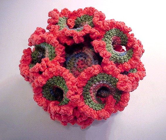
\[f^* g_{\text{Euc}} = (dx^2 + dy^2)/4 < dx^2 + \cosh^2(x) dy^2 = g,\]

hence \(f\) is a short embedding. By the Nash-Kuiper h-principle we can find a \(C^1\)-regular isometric embedding \(f_1 : (\Bbb R^2, g) \to \Bbb R^3\) which is \(C^0\)-close to \(f\), and thus as \(f\) is proper so is \(f_1\). We have found a proper \(C^1\)-regular isometric embedding of \(\Bbb H^2\) in \(\Bbb R^3\). The first embedding is a wild \(C^0\)-small perturbation of the Klein disk model, which essentially looks like a fractal-like ball of fuzz in space, almost like a hyperbolic crochet, with the ideal boundary \(\partial \Bbb{H}^2\) curled up into a wild continuum(?). On the other hand, the second example wrinkles more and more as we go towards infinity, to accommodate the exponential distance between points farther away from the origin.

At least two students of the said camp asked me if \(\Bbb H^2\) smoothly isometrically embeds in \(\Bbb R^n\) for some \(n > 3\). A non-explicit answer is given once again by Nash, which states that if \((M, g)\) is an arbitrary Riemannian \(n\)-manifold then there is a \(C^\infty\)-regular isometric embedding in \(\Bbb R^{n(n+1)(3n+11)/2}\). Plugging the numbers we find \(\Bbb H^2\) admits a smooth isometric embedding in \(\Bbb R^{51}\). This seems like a dauntingly high dimension, so an interesting question might be what the minimal dimension is. David Brander’s thesis, “Isometric Embeddings between Space Forms” includes a result of Danilo Blanuša which states \(\Bbb H^2\) admits a smooth isometric embedding in \(\Bbb R^6\). It’s a very clever construction which emphasizes a key idea in the easy half of Nash-Kuiper theorem (a topic for another day!), I think, so I will try to write down an expository of the proof.

We model \(\Bbb H^2\) by \((\Bbb R^2, g = dx^2 + \cosh^2(x) dy^2)\) as before. Our goal is to find an embedding \(f : \Bbb R^2 \to \Bbb R^6\) such that \(f^* g_{\mathrm{Euc}} = g\). Before stating the key lemma we go off on a tangent to make the following observation: Suppose \(\eta : \Bbb R \to \Bbb R\) is a \(C^\infty\)-function with bounded derivative. Consider the function \(F : \Bbb R^2 \to \Bbb R^2\),

\[\displaystyle F(x, y) = \left (\eta(x) \frac{\cos(cy)}{c}, \eta(x) \frac{\sin(cy)}{c} \right )\]

The function \(F\) essentially wraps the plane about itself so that the lines \(x = \mathrm{const}\) are mapped to circles of radius \(\eta(x)/c\) traversed in speed \(c\). It is an easy computation that

\[\displaystyle F^*(dx^2 + dy^2) = \frac{\eta'(x)^2}{c^2} dx^2 + \eta(x)^2 dy^2\]

If we let \(c \to \infty\), the angular coordinate is traversed so fast the radial direction contributes very little to the metric, and \(F^*(dx^2 + dy^2)\) becomes an arbitrarily good approximation of the quadratic differential \(\eta(x)^2 dy^2\). In fact, the bounded derivative hypothesis can be dealt away with by compromising more dimensions. Namely, let \(\psi = (\psi_1, \psi_2) : \Bbb R \to S^1\) be a smooth function such that \(\psi_i^{(k)}\) vanishes at the points congruent to \(i \pmod{2}\) for all \(k \geq 0\). Define \(F : \Bbb R^2 \to \Bbb R^4\) by

\[\displaystyle F(x, y) = \left ( \eta \psi_1 \frac{\cos(c_1 y)}{c_1}, \eta \psi_1 \frac{\sin(c_1 y)}{c_1}, \eta \psi_2 \frac{\cos(c_2 y)}{c_2}, \eta \psi_2 \frac{\cos(c_2 y)}{c_2} \right )\]

Where \(c_i\) are piecewise-constant functions, with jump discontinuities at the set of points congruent to \(i \pmod{2}\). Using \(\psi_1^2 + \psi_2^2 = 1\), we compute that

\[\displaystyle F^*(dx_1^2 + dx_2^2 + dx_3^2 + dx_4^2) = \left [ \left ( \frac{(\eta \psi_1)'}{c_1} \right )^2 + \left ( \frac{(\eta \psi_2)'}{c_2} \right )^2 \right ] dx^2 + \eta(x)^2 dy^2\]

We can now choose \(c_1, c_2\) appropriately large on each interval of continuity so that \(F^* g_{\mathrm{Euc}}\) is again an arbitrarily good approximation of \(\eta(x)^2 dy^2\). More precisely, we have \(F^* g_{\mathrm{Euc}} = \epsilon^2 dx^2 + \eta^2 dy^2\) where \(\epsilon = \epsilon(x)\) is small in \(C^0\)-norm. This trick crops up in the Nash-Kuiper theorem to “approximately immerse” a Riemannian manifold in a Euclidean space. I plan to discuss this in more detail elsewhere.

Consider the map \(f : \Bbb R^2 \to \Bbb R^6\), given by

\[f(x, y) = \left (\int_0^x \sqrt{1 - \epsilon(t)^2} dt, y, F(x, y) \right)\]

Then \(f\) is \(C^0\)-close to the parametrization of the graph of \(F\) which is an embedding, and by stability of embedings, we conclude \(f\) must be an embedding as well. Observe

\[f^*(g_\mathrm{Euc}) = (1 - \epsilon(x)^2) dx^2 + dy^2 + F^*(g_\mathrm{Euc}) = dx^2 + (1 + \eta(x)^2) dy^2\]

Plugging \(\eta(x) = \sinh(x)\) gives the required \(C^\infty\)-regular isometric embedding \(f : \Bbb H^2 \to \Bbb R^6\). Note also since the graph of \(F\) is properly embedded in \(\Bbb R^6\) and \(f\) is \(C^0\)-close to the graph, it is also a proper embedding. We can also use the approximation result on \(\eta(x) = \cosh(x)\) and let \(f : \Bbb R^2 \to \Bbb R^5\),

\[f(x, y) = \left (\int_0^x \sqrt{1 - \epsilon(t)^2} dt, F(x, y) \right),\]

forgetting the middle component. Then \(f^*(g_\mathrm{Euc}) = dx^2 + \eta^2(x) dy^2 = g\), so \(f\) is a \(C^\infty\)-isometric immersion of \(\Bbb H^2\) in \(\Bbb R^5\).

Whether the hyperbolic plane admits a \(C^k\)-isometric immersion in \(\Bbb R^4\) for \(k \geq 2\) is unknown, see Chapter 3.2 of Gromov, “Partial Differential Relations”.