Segue: a bit about foliations
Recall that a foliation on a three-manifold is a decomposition of the manifold as a union of continuum-many disjoint, possibly noncompact subsurfaces (called leaves of the foliation), so that locally the decomposition is the standard decomposition of the three-space as a union of affine subspaces given by level sets of a linear functional. An easy example of a foliation is given by fibers of a fiber bundle \(\pi : M \to S^1\) from the three-manifold onto the circle, but not all foliations are fibers of a fibration. A famous example is the Reeb foliation, which is a foliation of the solid torus \(S^1 \times D^2\) consisting a unique compact leaf given by the boundary torus, and the rest of the leaves are embedded planes spiraling around the torus, accumulating to the boundary leaf.
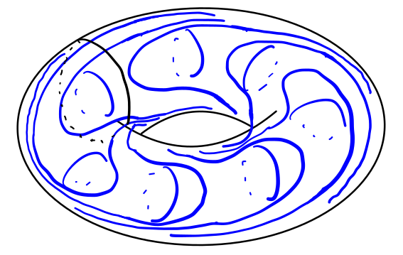
One may double the solid torus along the boundary by \((x, y) \mapsto (y, -x)\) to obtain an interesting foliation on \(S^3\). A general recipe to produce Reeb-like foliations is: suppose \(M\) is a manifold with torus boundary and \(\mathcal{F}\) be a foliation on \(M\) by surfaces with boundary, such that the boundary of the leaves themselves foliate the boundary of the manifold \(\partial M\). Then we may “spin” the leaves around the torus as we approach the boundary to obtain a foliation on \(M\) by the spun leaves of \(\mathcal{F}\) as well as a boundary leaf \(\partial M\). These are called dead-ends, since any arc transverse to the leaves foliation from the inside is stopped by the spinning leaves from ever intersecting the boundary leaf. One may also Dehn fill \(\partial M\) by a Reeb torus to obtain closed examples.
Theorem. Every three-manifold admits a foliation.
Proof. Choose an ambient Riemannian metric on \(M\). Since \(\chi(M) = 0\), there exists a nowhere zero vector field on \(M\). Taking the orthogonal complement at each point, we obtain a plane field \(\xi\). We wish to modify \(\xi\) to be everywhere integrable and thus give rise to a foliation. To this end, let \(\mathcal{T}= \cup_i \Delta_i^3\) be a triangulation of \(M\). We use the following lemma:
Lemma. (Thurston’s jiggling lemma) There exists a subdivision \(\mathcal{T}'\) of \(\mathcal{T}\) and a \(C^0\)-small perturbation \(\mathcal{T}''\) of \(\mathcal{T}'\) such that (1) \(\xi\) is transverse to the interiors of the edges and faces of \(\mathcal{T}''\) of \(\mathcal{T}'\) and (2) \(\xi\) is \(C^\infty\)-close to being horizontal on each \(3\)-simplex of \(\mathcal{T}''\) with respect to some affine coordinate system.
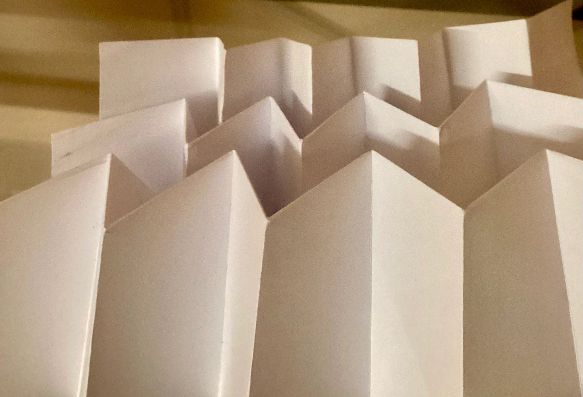
Proof of Lemma. First, barycentric subdivide \(\mathcal{T}\) until all simplices become of arbitrarily small diameter, i.e., \(\mathrm{diam}(\Delta_i^3) < \varepsilon\). Then by smoothness of \(\xi\), we may choose a coordinate system on each simplex with height coordinate \(z\) such that \(\xi\) is \(\varepsilon\)-close to \(\ker(dz)\). This ensures (2). Next, apply a crystalline subdivision procedure: embed \(\Delta^3\) in \([0, 1]^3\) as
\[\Delta^3 = \{(x, y, z) \in [0, 1]^3 : x + y + z \leq 1\}\]Then slice by the hyperplanes \(\{x = k/n\}\), \(\{y = k/n\}\) and \(\{x + y + z = k/n\}\). This subdivides the simplices into uniformly small simplices such that each vertex in the one-skeleton has bounded valence. Moving the vertices up and down by small rigid motions within \([0, 1]^3\), the entire crystalline-subdivided simplex crumples up in a way that all the smaller simplices in the crystalline subdivision are of large slope and therefore transverse to the plane field \(\xi \cong \ker(dz)\), ensuring (1) as well. In retrospect, the exact model of the subdivision process is not really important for this: see figure below.
Thus, by applying the jiggling lemma, we have made \(\xi\) transverse to the \(2\)-skeleton of the new triangulation \(\mathcal{T}''\), i.e., the “local min/max” with respect to \(\xi\) only occur at the vertices and possibly interiors of \(3\)-simplices. Remember that by construction, our \(2\)-plane field is co-oriented. Thus, the \(1\)-skeleton of the triangulation admits a directed graph structure, where we orient an edge so that it agrees with the co-orientation of the plane field. This also equips each simplex of the triangulation with a total order on the vertices so that all the edges point from a smaller vertex to a larger vertex. By a further subdivision of \(\mathcal{T}''\) if necessary, we can ensure that we can color the simplices red and blue so that adjacent simplices have different colors. We may tilt any particular red simplex so that the characteristic foliation has ``clockwise holonomy”, i.e., the leaves spiral down clockwise. Then on an adjacent blue simplex it spirals counterclockwise with respect to the natural coordinate system, by compatibility of orientation. This effect can then be inductively transported on all simplices.
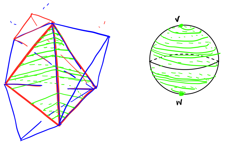
Intersect \(\xi\) with the \(2\)-skeleton of the triangulation. On each simplex, this leaves an imprint of the plane field which is a singular (combinatorial) foliation on the boundary of the \(2\)-simplex, which we will call the characteristic foliation. It consists of exactly one minimum at the largest vertex, one maximum at the smallest vertex, and spiraling leaves connecting between them. We may extend this foliation into a neighborhood of the \(2\)-skeleton. This gives a codimension \(0\) submanifold with spherical boundaries on which the singular foliation is as described before. We would like to fill these holes by balls. This seems impossible, because of the spiraling of the leaves in the characteristic foliation. So, for each three-simplex \(\Delta^3\) with maximum vertex \(v\) and minimum vertex \(w\), we find an arc \(\tau\) transverse to the foliation joining \(v, w\) outside \(\Delta^3\). If this was possible, we could delete a neighborhood of \(\tau\) to obtain a solid torus hole with a nonsingular characteristic foliation on the boundary. Then spinning and Reeb-filling finishes the proof.
It remains to show that such transverse arcs \(\tau\) can in fact be constructed. To do this, recall the color-coding of the three-simplices described a paragraph ago. Suppose \(\Delta^3\) is a red simplex. Then the characteristic foliation has clockwise holonomy. The strategy is to take an arc \(\tau\) joining \(v, w\) in \(\partial \Delta^3\) transverse to the singular foliation with anti-clockwise holonomy, so that it is transverse to all the leaves. Then we could take a push-off of \(\tau\) so that the interior of \(\tau\) is disjoint from \(\Delta^3\).
This has a problem, in that the picture of the characteristic foliation in the above figure is ``wrong”. If the characteristic foliation was infinitely spiraling near the max/min vertices \(v, w\) as in the picture, we would not be able to extend it inwards on a regular neighborhood because of the singularity. We need to modify the plane field (or the coordinate system) so that near \(v, w\) the characteristic foliation is by concentric circles (or triangles, before smoothening), and outside a little neighborhood we have the spiraling pattern, to be able to extend to a smooth foliation in a regular neighborhood of the \(2-\)skeleton. But now we have a problem with constructing the arc \(\tau\) near \(v, w\). To solve this problem, we observe that there is an adjacent blue simplex such that \(v, w\) are one of the non-extremal vertices of this simplex. We start the arc \(\tau\) by going from \(v\) into this adjacent simplex, spiral downwards in counterclockwise fashion by following the singular foliation, come back to \(\Delta^3\) and follow our transverse arc counterclockwise to the characteristic foliation on \(\partial \Delta^3\), and once we are sufficiently close to \(w\), go back out into the adjacent simplex and follow its characteristic foliation again until coming back to \(w\) from the outside. Taking a push-off of this satisfies the required transversality property.
Remark. An analogous proof shows that all three-manifolds admit a contact structure, but its easier because the figure above for the characteristic foliation on the sphere is not wrong, and finding transverse arcs are much easier in contact topology. This also shows that any plane field can be homotoped to a foliation (respectively, contact structure). See, “Confoliations” by Thurston and Eliashberg for more.
OK, every three-manifold has a foliation. But what if we changed the rules so that you cannot cheat?
Definition. A foliation \(\mathcal{F}\) is taut if there exists an closed curve \(\gamma\) transversely intersecting all the leaves of \(\mathcal{F}\).
This immediately rules out existence of Reeb components and dead-end components. So the proof above, which heavily relied on filling toroidal holes by Reeb foliations, breaks completely. So which three-manifolds admit taut foliations? Some immediate examples are that of fibered manifolds in the beginning of the post. We give an example of a taut foliation which is not fibered.
Example. Let \(f : \Sigma \to \Sigma\) be a diffeomorphism of a surface of genus \(g \geq 2\). Let \(M = T(f)\) be the mapping torus of \(f\), which admits an obvious fibering \(\pi : M \to S^1\) by construction. We shall modify the fibering to be a rather complicated taut foliation, as follows. Consider \(\Sigma \times [0, 1]\) with the standard foliation by \(\Sigma \times \{x\}\). Let \(C \subset \Sigma\) be any non-separating essential curve, for instance, a meridian. Then the annulus \(C \times [0, 1]\) intersects all the leaves of the standard height foliation transversely. We cut \(\Sigma \times [0, 1]\) open along \(C \times [0, 1]\), so that every leaf becomes a surface of genus \(1\) with two punctures.
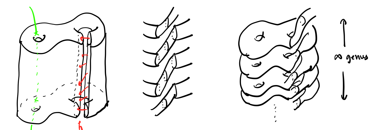
Let \(h : [0, 1] \to [0, 1]\) be a homeomorphism such that \(0, 1\) are fixed points of \(h\), such that \(0\) is an attracting fixed point. We now ``cross-glue” the cut open \(\Sigma \times [0, 1]\) along \(C \times [0, 1]\) by \(h\), so that the cut-open leaves at different heights glue among themselves. Since \(h(0) = 0\) is an attracting fixed points, we will see infinite-genus surface leaves accumulating to \(\Sigma \times \{0\}\) in the resulting foliation. We glue the top and bottom by \(f\) to get back \(M\) with a new foliation that is definitely not fibered. Moreover, since the cutting-repasting operation does nothing to the foliation on one side, there is a closed transversal all the same: see the green arc above.
However, this only gives examples of interesting taut foliations on the class of fibered three-manifolds. Eventually, I would like to describe Gabai’s construction of taut foliations on many more three-manifolds (in fact, one just needs the first betti number to be positive). For now, in the next post we shall discuss the geometry of taut foliations: Sullivan’s theorem (topologically taut implies geometrically taut) and what it has to do with max-flow-min-cut. And then return to the Thurston norm, eventually.