Seiberg-Witten Theory: II
Recall from the last paragraph of Part I that we wished to carry out all of the linear algebra but now parametrized over a manifold \(M\). Let us try to naively carry out the procedure, and in the process we will encounter the issue: let \((M, g)\) be a Riemannian \(n\)-manifold where \(n = 2m\) is even. The Riemannian metric \(g\) is a smoothly-varying inner product on each tangent space \(T_p M\), \(p \in M\) which assemble to the tangent bundle \(TM\), so one can take the Clifford algebra \(\mathrm{Cliff}(T_p M, g_p)\) for each \(p \in M\) and assemble these to a “Clifford algebra bundle” \(\mathrm{Cliff}(M) := \mathrm{Cliff}(TM, g)\). One can try to construct a fiberwise complex spinor representation, which would be a bundle \(S\) over \(M\) such that for each \(p \in M\), \(S_p\) is the complex spinor representation of \(\mathrm{Cliff}(T_pM, g_p)\); this we know how to construct, simply look at the complexification \(T_p^{\Bbb C} M := T_p M \otimes \Bbb C\) with the complexified inner product \(g^{\Bbb C}_p := g_p \otimes \Bbb C\) (which is a symmetric bilinear form, not a Hermitian inner product), take \(\mathrm{Cliff}^{\Bbb C}(T_p M, g_p) := \mathrm{Cliff}(T_p^{\Bbb C} M, g^{\Bbb C}_p)\) the complex Clifford algebra (which is in fact the complexification of the real Clifford algebra as described before in Part I) which assemble to the complex Clifford bundle \(\mathrm{Cliff}^{\Bbb C}(M)\), look at its action on the exterior algebra over the maximal totally isotropic subspace (or “Lagrangian subspace” in symplectic geometry terminology) of \(T_p^{\Bbb C} M\) as described previously, and that’s exactly \(S_p\). Assemble these up and we are done…
Except, to construct the maximal isotropic, we needed an extra piece of data, a choice of an orthogonal almost-complex structure or a transformation \(J_p : T_p M \to T_p M\) such that \(J_p^2 = -I\) and \(J_p\) is an isometry with respect to \(g_p\); the eigenspace corresponding to the eigenvalue \(i\) of \(J_p\) on \(T_p^{\Bbb C} M\) is the maximal isotropic. This extra piece of data is not just a random choice that we can make; to assemble everything to a bundle at the end, we need a smoothly varying family of almost-complex structures on each tangent space of \(M\), i.e., a metric-compatible, fiberwise almost complex structure \(J : TM \to TM\), \(J^2 = -I\). Existence of such a thing is not automatic, in fact they do not always exist. Kahler manifolds (eg, smooth zero loci of homogeneous equations treated as subsets of \(\Bbb{CP}^n\)) are examples of such things, in fact they are exactly the ones for which this \(J\) is integrable in the sense that it gives rise to complex coordinate charts on the manifold; integrability is a closed condition \(J\) (the Nijenhuis tensor vanishes) so certainly Kahler manifolds are a rarer class than we are looking for. So what exactly are the Riemannian manifolds \((M, g)\) which admit an orthogonal almost-complex structure? Define \(\omega(X, Y) = g(X, JY)\) and observe that \(\omega\) is a \(2\)-form on \(M\), and moreover \(\omega^m := \omega \wedge \cdots \wedge \omega\) is a nowhere vanishing volume form on \(M\). Thus, \(\omega\) is an almost-symplectic structure, the difference from an actual symplectic structure being again an integrability condition: \(d\omega = 0\) or closedness of \(\omega\). On the other hand if \(M\) was an almost-symplectic manifold, the form \(\omega\) assumed to have no apriori compatibility with \(g\), one could have constructed an orthogonal almost-complex structure by the polar decomposition formula: \(J = (\Omega^{\mathsf{T}} \Omega)^{-1/2}\Omega\) where \(\Omega\) denotes the matrix of the bilinear form \(\omega\) with respect to some \(g\)-orthonormal basis; these are the so-called \(\omega\)-compatible almost complex structures (particularly relevant when \(\omega\) is symplectic, in the theory of pseudoholomorphic curves). In any case, we see that the class of manifolds we are interested in is larger, even, than symplectic manifolds.
Nonetheless, they are not abundant. The only spheres which admit an almost-complex structures are \(S^2\) and \(S^6\). Indeed, suppose \(TS^{2n}\) admits an almost complex structure \(J\). Then \(J \otimes \Bbb C\) gives an eigendecomposition of complex vector bundles \(T^{\Bbb C} S^{2n} = E \oplus \overline{E}\) where \(E = TS^{2n}\) with the complex structure \(J\), and \(\overline{E}\) is the conjugate. We compute the Chern class \(c_n\) of either side; note that \(c_n(T^{\Bbb C} S^{2n}) = 0\) by complex stable triviality of the complexified tangent bundle of the sphere, and \(c_n(E \oplus \overline{E}) = c_n(E) + c_n(\overline{E})\). If \(n\) was even, this would be \(2c_n(E) = 2\chi(S^{2n})[S^{2n}] = 4[S^{2n}]\), which gives the required contradiction. Note that the argument here is really a Pontryagin class argument, \(p_k(S^{4k}) = c_{2k}(T^{\Bbb C} S^{4k})\). Indeed, if \(k = 1\), then \(p_1(S^4) = 0\) can be seen geometrically, since by Chern-Weil theory \(p_1(M) = 1/(8\pi^2) \int_M \mathrm{tr}(\Omega^2)\) where \(\Omega\) is the curvature \(2\)-form of some chosen Riemannian metric on \(M\). If \(M\), like the sphere, admits a metric of constant curvature \(K\), then \(\Omega_{ij} = K d\omega^i \wedge d\omega^j\) which implies \(\Omega^2\) has no diagonal terms and so the \(1\)st Pontryagin form itself is zero. In the case \(n\) is odd, the above procedure gives no contradiction as \(c_n(\overline{E}) = -c_n(E)\); we can instead argue by Chern classes modulo \(p\) for some odd prime \(p\): from here, we see if \(n - p + 1 > 0\), the universal Chern classes modulo \(p\), \(c_n \pmod{p}\) can be written as a polynomial in \(c_1 \pmod{p}, \cdots, c_{n-1} \pmod{p}\) and the first Steenrod power \(P^1(c_{n-p+1} \pmod{p})\). Specializing to \(TS^{2n}\) we get that since \(c_i = 0\) for all \(i < n\), \(c_n(TS^{2n}) = 2[S^{2n}] \pmod{p} = 0\), which would be a contradiction. For this, we require an odd prime \(p\) such that \(p < n - 1\), that is, \(n > 4\). This leaves the cases \(n = 1, 2, 3, 4\) and \(n = 2, 4\) are eliminated by the earlier argument with the Pontryagin class. Thus, \(n = 1, 3\) are the only possibilities and these in fact do admit almost complex structure; whether \(S^6\) admits an integrable almost complex structure is still an open problem.
Here’s the punchline. You do not actually need an almost complex structure to get a spinor bundle, all you need is a much weaker spinc structure. My understanding is that the story of spin geometry begins with trying to “soften” almost complex geometry; almost complex structures are rare, so we would like to enlarge the tangent bundle to the “spinor bundle” where almost complex structures are abundant.
Let’s organize what we did in Part I from this viewpoint; given a real inner product space \((V, \langle \cdot, \cdot \rangle)\), we are interested in studying Clifford modules \(W\) over \(V\) which is a Hermitian inner product space \(W\) on which \(V\) acts in a way that each unit vector \(v \in V\) acts by an almost complex structure \(J_v : W \to W\), i.e., \(J_v^2 = -I\) and for any pair \(u, v \in V\) of unit vectors, \(J_u J_v = -J_v J_u\). That is to say, \(W\) is an enlargement of \(V\) which admit the unit sphere in \(V\)’s worth of almost-complex structures which are all compatible (i.e., for any pair of unit vectors \(u, v\), the complex structures \(I, J_u, J_v, J_u J_v\) form a linear almost-hyperKahler structure on \(W\)). The subalgebra of \(\mathrm{End}(W)\) generated by \(\{J_v : v \in V, \|v\| = 1\}\) is the (actual, physically perceivable) Clifford algebra \(\mathrm{Cliff}(V) \subset \mathrm{End}(W)\); one simply identifies \(v\) with \(J_v\) and composition of operators is the Clifford product, so \(V\) sits inside its Clifford algebra as the degree \(1\) elements. Next, observe that the axioms of the Clifford algebra implies for any pair of orthogonal unit vectors \(u, v\in V\), \(-vuv^{-1} = u\) unless \(u = \pm v\) in which case \(-vuv^{-1} = -u\). Define
\[\begin{gather*}\mathrm{ad} : \mathrm{Cliff}(V)^\times \to \mathrm{End}(\mathrm{Cliff}(V)),\\ \mathrm{ad}_\alpha(u) = -\alpha u \alpha^{-1}\end{gather*}\]Observe that \(\mathrm{ad}_v(V) \subset V\) if \(v\) is a degree \(1\) element by our observation before. In fact, we get also from our observation that if \(\|v\| = 1\) then \(\mathrm{ad}_v\) is reflection along the hyperplane \(\langle v \rangle^\perp\). Thus, define,
\[\displaystyle \begin{align*}\mathrm{Pin}(V) &= \{v_1 \cdots v_k \in \mathrm{Cliff}(V) : v_i \in V, \|v_i\| = 1\} \\ \mathrm{Spin}(V) &= \mathrm{Pin}(V) \cap \mathrm{Cliff}^+(V)\end{align*}\]These are both subgroups of \(\mathrm{Cliff}(V)^\times\), and the adjoint representation restricts to homomorphisms (caveat: this doesn’t quite work, but the lie will be explained below) \(\mathrm{ad} : \mathrm{Pin}(V) \to \mathrm{O}(V)\) and \(\mathrm{ad} : \mathrm{Spin}(V) \to \mathrm{SO}(V)\) (here we are using that every orthogonal transformation is a product of reflections) which are \(2:1\) because \(\langle v \rangle^\perp = \langle -v\rangle^\perp\) so the reflections \(\mathrm{ad}_v\) and \(\mathrm{ad}_{-v}\) are the same. In fact they are both covering maps, and \(\mathrm{ad} : \mathrm{Spin}(V) \to \mathrm{SO}(V)\) is the universal cover.
There is an alternative description of these groups: consider the involution \(*\) on \(\mathrm{Cliff}(V)\) which acts on degree \(1\) elements by \(v^* := -\overline{v}\) and extending to monomials by reversing order: \((v_1 \cdots v_k)^* = v_k^* \cdots v_1^*\). The spinor norm is defined by \(\\|x\\| = x^* x\); observe on degree \(1\) elements this coincides with the norm coming from the inner product, and \(\\|xy\\| = \\|x\\| \\|y\\|\) follows from the definition. Thus, products of unit norm elements of \(V\) is contained in the unit sphere of \(\mathrm{Cliff}(V)\) under this norm, hence so is \(\mathrm{Pin}(V)\). But it is possible to have non-monomial elements in the unit sphere as well; to eliminate these we need the extra condition that \(x^* V x = V\). Indeed, then \(\mathrm{ad}_x \in \mathrm{O}(V)\) hence \(x \in \mathrm{Pin}(V)\) is forced. Therefore,
\[\displaystyle \mathrm{Pin}(V) = \{x \in \mathrm{Cliff}(V) : \\|x\\| = 1, x^* V x = V\}\]and \(\mathrm{Spin}(V) = \mathrm{Pin}(V) \cap \mathrm{Cliff}^+(V)\) as before. Now we are in a position to explain the lie in the definition of the double cover \(\mathrm{Pin}(V) \to \mathrm{O}(V)\) above; the adjoint action \(\mathrm{ad}_x(u) = -xux^*\) is not a homomorphism in \(x\) from the full pin group. Indeed, \(\mathrm{ad}_x \circ \mathrm{ad}_{x'} = -\mathrm{ad}_{xx'}\); one has to correct for signs here, one of the many woes of working in a superalgebra. One way to do it is to taint an element with negative sign in odd degrees and positive sign in even degrees. Then \(\mathrm{ad}_x(v) := (-1)^{\|x\|} x v x^*\) works perfectly fine and agrees with the usual adjoint on the spin group, where sign is a non-issue as it lives in even degrees.
So far all we have talked about is the real Clifford algebra. The complex Clifford algebra is just obtained from tensoring everything up with \(\otimes_{\Bbb R} \Bbb C\); the last definition of the pin group goes through in this setup provided we complexify \(*\) correctly: define \(v^* = -\overline{v}\) in degree \(1\) instead; note that the conjugation only affects the scalars that hang around because of extending scalars to \(\Bbb C\) in the definition of the complex Clifford algebra, not the vectors themselves (remember the inner product on \(V \otimes \Bbb C\) is still a symmetric bilinear form, not a Hermitian one). We call the resulting groups \(\mathrm{Pin}^{\Bbb C}(V)\) and \(\mathrm{Spin}^{\Bbb C}(V)\). Explicity,
\[\displaystyle \begin{align*}\mathrm{Pin}^{\Bbb C}(V) &= \{e^{i\theta} x \in \mathrm{Cliff}^{\Bbb C}(V) : x \in \mathrm{Pin}(V)\} \\ \mathrm{Spin}^{\Bbb C}(V) &= \{e^{i\theta} x \in \mathrm{Cliff}^{\Bbb C}(V) : x \in \mathrm{Spin}(V)\}\end{align*}\]This time \(\mathrm{ad} : \mathrm{Pin}^{\Bbb C}(V) \to \mathrm{O}(V)\) and \(\mathrm{ad} : \mathrm{Spin}^{\Bbb C}(V) \to \mathrm{SO}(V)\) have kernel \(S^1 \cong U(1)\). From the concrete description of the spin group above, we see \(\mathrm{Spin}^{\Bbb C}(V)\) is almost \(U(1) \times \mathrm{Spin}(V)\), except \(\pm 1\) can appear in either factor, which leads to a \(\Bbb Z/2\)-ambiguity. Thus, \(\mathrm{Spin}^{\Bbb C}(V) \cong U(1) \times_{\Bbb Z/2} \mathrm{Spin}(V)\). As a consequence, \(\mathrm{Spin}^{\Bbb C}(V)\) can also be thought as a double cover of \(U(1) \times \mathrm{SO}(V)\).
The real usage of complexifying everything up is that the representation theory of \(\mathrm{Cliff}^{\Bbb C}(V)\) is simpler than that of \(\mathrm{Cliff}(V)\). This is not strictly speaking relevant to us, but just to explain that comment I will go into a very brief detour: our focus has so far been on even-dimensional \(V\) but more or less everything discussed above goes through in odd-dimensions as well (however, \(\mathrm{Cliff}^{\Bbb C}(V)\) for odd dimensional \(V\) has two irreducible representations). Then for every \(n\) we have the Clifford algebras \(\mathrm{Cliff}(n)\) (what we called \(\mathrm{Cliff}_{n, 0}\) in Part I) and \(\mathrm{Cliff}^{\Bbb C}(n)\). But as it happens, there is a periodicity in the structure of these algebras: the complex Clifford algebras are \(2\)-periodic in the sense that \(\mathrm{Cliff}^{\Bbb C}(n+2) = M_2(\mathrm{Cliff}^{\Bbb C}(n))\) whereas the real Clifford algebras happen to be \(8\)-periodic, i.e., \(\mathrm{Cliff}(n+8) = M_{16}(\mathrm{Cliff}(n))\). \(\mathrm{Cliff}^{\Bbb C}(n)\) is always either a matrix algebra (on its unique complex spinor representation) or a product of two matrix algebras (in case \(n\) is odd). But \(\mathrm{Cliff}(n)\) form the complicated Bott tower: the first eight algebras starting from \(n = 0\) are
\[\displaystyle \Bbb R, \Bbb C, \Bbb H, \Bbb H \oplus \Bbb H, M_2(\Bbb H), M_4(\Bbb C), M_8(\Bbb R), M_8(\Bbb R) \oplus M_8(\Bbb R)\]One should conceptualize this as a linear version of the topological Bott periodicty, one of many ways of stating which is that the homotopy groups of \(O(\infty)\) are \(8\)-periodic.
Let me mention a modest, but illuminating example. \(\mathrm{Cliff}(3)\) is generated by \(e_1, e_2, e_3\), the full graded algebra breaks into four parts \(\mathrm{Cliff}_0 \oplus \mathrm{Cliff}_1 \oplus \mathrm{Cliff}_2 \oplus \mathrm{Cliff}_3\) indexed by degree. The degree \(2\) part is generated by \(e_1 e_2, e_2 e_3, e_3 e_1\) which can be sent to the quaternions \(i, j, k\); hence, there is an embedding \(\Bbb H \cong \mathrm{Cliff}(2) \hookrightarrow \mathrm{Cliff}(3)\) as the degree \(2\) elements (more generally, \(\mathrm{Cliff}(n-1)\) embeds in \(\mathrm{Cliff}(n)\) as the degree \(n-1\) elements). The degree \(0\) and \(3\) parts are both \(1\)-dimensional, the latter generated by \(e_1 e_2 e_3\). The \(\mathrm{Spin}(3)\) group lives inside the even degree part which is \(\mathrm{Cliff}_0 \oplus \mathrm{Cliff}_2 = \Bbb R \oplus i \Bbb H = \Bbb H\), consisting of all the elements of unit norm, i.e., \(\mathrm{Spin}(3) \cong S^3 \cong \mathrm{SU}(2)\). It is a classical fact that conjugation by a quaternion are rotations in the \(i\Bbb H\) factor, so this gives
\[\mathrm{ad} : \mathrm{Spin}(3) \cong \mathrm{SU}(2) \to \mathrm{SO}(3)\]It is tempting to try to figure out \(\mathrm{Spin}(4)\) as well. From the Bott tower above we can see
\[\mathrm{Cliff}(4) \cong \Bbb H \oplus \Bbb H\]This is in fact a \(*\)-algebra isomorphism. The unit sphere then is \(\mathrm{SU}(2) \times \mathrm{SU}(2)\). So, we have
\[\mathrm{Spin}(4) \subseteq \mathrm{SU}(2) \times \mathrm{SU}(2)\]The equality holds as there is a \(2 : 1\) map \(\mathrm{SU}(2) \times \mathrm{SU}(2) \to \mathrm{SO}(4)\) given by \((q_1, q_2) \mapsto (u \mapsto q_1 u \overline{q_2})\), and the kernel is \(\Bbb Z/2 \cong \{(1, 1), (-1, -1)\}\). I haven’t quite worked out the details of how it fits together with the linear algebra of \(\mathrm{Cliff}(4)\), though.
The final piece of linear algebra that I want to discuss in this post is about how the complex Clifford algebra, the complex spinor representation and the spin group are tied together. First, observe (say, using Schur’s lemma) that \(\mathrm{End}_{\Bbb C}(S) \cong \mathrm{Cliff}^{\Bbb C}(V)\), so the Clifford algebra is completely recovered from the complex spinor representation. Next, consider the spinc automorphisms of \(S\), i.e., a pair of transformations \(A : V \to V\) and \(T : S \to S\) such that \(A\) is orthogonal and \(T\) is unitary, such that \(T \circ \rho \circ T^{-1} = \rho \circ A\) where \(\rho : V \to \mathrm{End}(S)\) is the (reified, i.e., in degree \(1\)) Clifford representation. Then we claim \(\mathrm{Aut}_{\mathrm{Spin}^{\Bbb C}}(S) \cong \mathrm{Spin}^{\Bbb C}(V)\), so that the spin group is also recoverable from the complex spinor representation. Indeed, \(T \in \mathrm{End}(S) \cong \mathrm{Cliff}^{\Bbb C}(V)\) hence \(T = \rho(x)\) for some \(x \in \mathrm{Cliff}^{\Bbb C}(V)\). Unitarity of \(T\) implies \(\\|x\\| = 1\); moreover the condition implies \(\rho(x^* v x) = \rho(A v)\) for all \(v \in V\). But \(\rho : \mathrm{Cliff}(V) \to \mathrm{End}(S)\) is an isomorphism so \(x^*vx = Av\). Therefore, \(\mathrm{ad}_x(V) = V\), but also \(\mathrm{ad}_x\) is an orientation-preserving transformation of \(V\). This implies \(x\) is in fact even, and so \(x \in \mathrm{Spin}^{\Bbb C}(V)\), which proves the claim. Finally, the complex spinor representation itself can be restricted to the group \(\mathrm{Spin}^{\Bbb C}(V) \subset \mathrm{Cliff}^{\Bbb C}(V)\) from the full Clifford algebra, which gives a representation, also called the complex spinor representation, \(\mathrm{Spin}^{\Bbb C}(V) \to \mathrm{End}(S)\). Recall in the case \(\dim V\) was even, we had defined a splitting \(S = S^+ \oplus S^-\) into the eigenspaces of the volume form on \(V\) and degree \(1\) elements acted on the decomposition by switching \(S^+, S^-\). As \(\mathrm{Spin}^{\Bbb C}(V)\) consists only even elements, we obtain that the representation over the spin group splits as \(S^+ \oplus S^-\); it is a fact that \(S^{\pm}\) are irreducible representations of \(\mathrm{Spin}^{\Bbb C}(V)\).
Here is how all of this ties the topological setup that was being discussed in the first couple of paragraphs in the beginning of the post. Suppose that \(S\) is a spinor bundle over a Riemannian manifold \((M, g)\) of dimension \(n = 2m\). Consider the model spinc structure \(\rho_0 : \Bbb R^n \to \mathrm{End}(\Bbb C^{2^m})\) that was discussed in Part I. Then define a principal \(\mathrm{Spin}^{\Bbb C}(n)\)-bundle \(P_\rho \to M\) whose fiber over \(p \in M\) consists of all the spinc isomorphisms between \(\rho_0\) and \(\rho_p : T_p M \to \mathrm{End}(S_x)\); that is:
\[\displaystyle P_\rho = \{(p, A, T) : A \in \mathrm{Isom}(\Bbb R^n, S_p), T \in \mathrm{Isom}(\Bbb C^{2^m}, S), T \circ \rho_0 \circ T^{-1} = \rho \circ A\}\]with \(\mathrm{Spin}^{\Bbb C}(n)\) acting by \(\alpha \cdot (p, A, T) = (p, A \circ \mathrm{ad}_\alpha, T \circ \rho_0(\alpha))\). If we forget the factor of \(T\) then this is simply the orthonormal frame bundle \(\mathrm{Fr}(M) \to M\), fiber of a generic point \(p\) of which is simply the space of all possible frames of \(T_p M\), and \(\mathrm{Spin}^{\Bbb C}(n)\) acts non-effectively by the projection \(\mathrm{Spin}^{\Bbb C}(n) \to \mathrm{SO}(n)\) to the group of orthogonal transformations, which simply permute the frames around over any given point. Remembering the spinor representation in the definition has the effect that the “spin” (whatever that is, more on this below) of the framing is remembered. In fact, consider \(P_\rho \times_{\mathrm{ad}} \mathrm{SO}(n) = (P \times \mathrm{SO}(n))/\mathrm{Spin}^{\Bbb C}(n)\) where \(\mathrm{Spin}^{\Bbb C}(n)\) acts diagonally, on \(P\) by permuting the spin framings and on \(\Bbb R^n\) by \(\mathrm{ad}\). Then it is clear that \(P_\rho \times_{\mathrm{ad}} \mathrm{SO}(n) \cong \mathrm{Fr}(M)\), as one is collapsing down the \(T\) factor (“spin”) wherever they record more information than the \(A\) factor (“frames”), so one just ends up with the frames. This is an incredibly concise way of putting the idea of spinor bundles, and it is clear with a little though that one can go the other way as well; if there was a \(\mathrm{Spin}^{\Bbb C}(n)\)-equivariant map \(P \to \mathrm{Fr}(M)\) from some principal \(\mathrm{Spin}^{\Bbb C}(n)\)-bundle to the frame bundle, one could take \(P \times_{\rho_0} \Bbb{C}^{2^m}\) to get back the spinor representation, where \(\rho_0 : \mathrm{Spin}^{\Bbb C}(n) \to M_{2^m}(\Bbb C)\) is the restriction of the model spinor representation to the spinc subgroup. All of this goes through likewise for real spinor representations as well, and parity of dimension of \(M\) is a mere convenience.
Definition. A spinc structure on an oriented Riemannian manifold \((M^n, g)\) is a principal \(\mathrm{Spin}^{\Bbb C}(n)\)-bundle \(P \to M\) such that \(P \times_{\mathrm{ad}} \mathrm{SO}(n) \cong \mathrm{Fr}(M)\). Likewise, a spin structure is a principal \(\mathrm{Spin}(n)\)-bundle \(P \to M\) such that \(P \times_{\mathrm{ad}} \mathrm{SO}(n) \cong \mathrm{Fr}(M)\).
We have proved that admitting a (complex) spinor representation is equivalent to admitting a spinc structure. I will demonstrate that this is far, far more flexible a condition than admitting an almost complex structure, but before that I would like to present some pictures which puts it in an intuitive and handwavy way; after all, for much of the time we have been doing abstract linear algebra and it might seem at first that spin structures emerge out of playing such algebraic games. I would like to argue, on the contrary, that it “actually exists” and something whose presence “can be felt”.
Let me discuss the real spin structure. Recall \(\mathrm{Spin}(n)\) is the universal double cover of \(\mathrm{SO}(n)\). For any nice topological group \(G\) the universal cover can be written as follows:
\[\widetilde{G} = \{\gamma \in \mathrm{Maps}([0, 1], G) : \gamma(0) = e\}/\sim\]where \(\sim\) denotes homotopy relative to the basepoint \(0\). The covering projection \(\widetilde{G} \to G\) is \(\gamma \mapsto \gamma(1)\). Now, there is a group structure on \(\widetilde{G}\) which is given by \((\alpha \beta)(t) = \alpha(t) \beta(t)\) and this is the one which lifts the group structure on \(G\). However, it is equivalent to the group structure given by \(\alpha * (\alpha(1)\beta)\) where \(*\) denotes path concatenation, as can be seen by hand. Specialize to the case \(G = \mathrm{SO}(n)\), which tells you elements of \(\mathrm{Spin}(n)\) are paths in \(\mathrm{SO}(n)\) starting at the identity, with multiplication of two such paths given by translating the initial point to the endpoint of the other, and then concatenating.
To visualize this with \(n = 3\), consider the following artifice. Consider a sphere \(S^2 \subset \Bbb R^3\) with an infinite strip (or a framed, proper ray) attached to it, which has red markings by arrows pointing up:
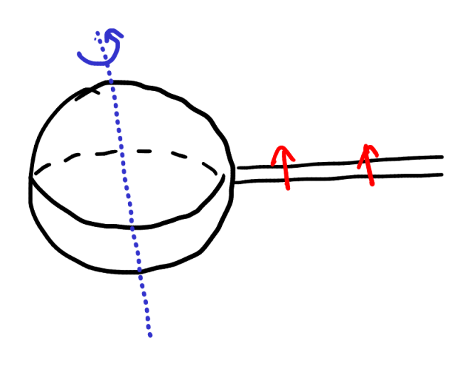
\(\mathrm{SO}(3)\) acts on the sphere by rotating it, but when we physically carry out a rotation we will have to follow a path of rotations starting at the identity and leading to the required rotation; the purpose of the strip is to keep track of this path “in space” rather than “in time”. For example, this is the effect of rotating the sphere by \(2\pi\) around the blue axis, which is the identity operation but as the strip tells you, that path you traced out is a nontrivial loop in \(\mathrm{SO}(3)\).
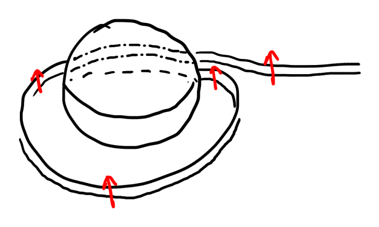
Indeed, try to unravel the strip out by moving it to one side as it was before, and one ends up with the following configuration:
We see one of the red arrows pointing down, in other words a full twist in the strip. If we do it again, we might see either two full twists or none, depending on how we unravel the strip and bring it to one side - I encourage carrying this out by cutting out some paper strips. Therefore, it makes sense to count the number of twists on the strip modulo 2, i.e., the strip can have only two states, an “up” state and a “down” state, corresponding to any state of the sphere. This is exactly how elements of \(\mathrm{Spin}(3)\) look like. This description of the spin group is not new; it is called the Dirac’s belt/plate trick. An elaborate animation can be found here where many such strips or belts are emerging out of the object that is exhibiting rotation.
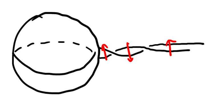
I think of a spin structure on a manifold \(M\) as a collection of such strips or framed proper rays from infinity attached to each unit tangent sphere so that the manifold looks like a marionette, and the associated “spin field” is the signed count of the number of full-twists or the up/down states along the strings. Probably not very useful, but sort of pleasant.
Finally, let us get to exactly what kind of topological obstructions there are for a spin or spinc structure on a manifold to exist. Off the top of my head, here is a way to do this by throwing the kitchen sink at it: the frame bundle of \(M\) is classified by a map \(M \to B\mathrm{SO}(n)\), and the question of admitting a spin or spinc structure is the same question as lifting this to a map \(\psi : M \to B\mathrm{Spin}(n)\) or \(M \to B\mathrm{Spin}^{\Bbb C}(n)\) respectively. In the first case, there is a fibration sequence \(\mathrm{SO}(n) \to \mathrm{Spin}(n) \to B\Bbb Z/2\) where the last map classifies the first map, which is a double covering. By delooping everything, we get a fibration sequence \(B\mathrm{SO}(n) \to B\mathrm{Spin}(n) \to B^2\Bbb Z/2\). Thus, the question of lifting a map from \(M\) to the middle term to a map into the fiber is equivalent to the question of whether the composition \(M \to B^2 \Bbb Z/2\) to the base is nullhomotopic. This is classified by an element of \(H^2(M; \Bbb Z/2)\); moreover it follows that this element lies in the image of the homomorphism \(\psi^* : H^2(B\mathrm{SO}(n); \Bbb Z/2) \to H^2(M; \Bbb Z/2)\). As explained in this post, the cohomology ring \(H^*(B\mathrm{SO}(n); \Bbb F_2) = \Bbb F_2[w_1, w_2, \cdots, w_n]\) is generated by universal Stiefel-Whitney classes, hence the unique nonzero element in degree \(2\) is \(w_2\). Thus, the class in \(H^2(M; \Bbb Z/2)\) is the second Stiefel-Whitney class \(w_2(M)\). In the second case, there is a fibration sequence \(\mathrm{Spin}^{\Bbb C}(n) \to \mathrm{SO}(n) \to BU(1)\) which one can deloop as before and argue that the relevant obstruction for lifting \(\psi\) to \(M \to B\mathrm{Spin}^{\Bbb C}(n)\) lies in \(H^3(M; \Bbb Z)\). Apparently, the class here is the “3rd integral Stiefel-Whitney class” \(W_3 := \beta w_2\), where \(\beta : H^2(-; \Bbb F_2) \to H^3(-; \Bbb Z)\) is the integral Bockstein in degree \(2\), which looks intuitive enough but I haven’t worked out precisely why. Moreover, it might be worth phrasing all of this in terms of explicit cocycles than abstract obstruction theory.
Edit: I have figured out why the obstruction class is \(W_3 = \beta w_2\). There is a short exact sequence
\[0 \to \Bbb Z/2 \to \mathrm{Spin}^{\Bbb C}(n) \to \mathrm{SO}(n) \times \mathrm{U}(1) \to 0\]which is classified by an element of \(H^2(\mathrm{SO}(n) \times \mathrm{U}(1); \Bbb Z/2) \cong H^2(\mathrm{SO}(n); \Bbb Z/2) \oplus H^2(\mathrm{U}(1); \Bbb Z/2)\) whose projection to the first factor classifies the short exact sequence
\[0 \to \Bbb Z/2 \to \mathrm{Spin}(n) \stackrel{\mathrm{ad}}{\to} \mathrm{SO}(n) \to 0\]obtained from the above short exact sequence by “forgetting the complex scalars” and the projection to the second factor classifies the short exact sequence
\[0 \to \Bbb Z/2 \to U(1) \stackrel{\times 2}{\to} U(1)\]obtained from the same short exact sequence by “forgetting the orthogonal matrices”. Therefore, the pertaining element of \(H^2(\mathrm{SO}(n); \Bbb Z/2)\) is \(w_2\) and let us call the element in \(H^2(U(1); \Bbb Z/2)\) as \(\alpha\). Thus, the classifying element is \(w_1 + \alpha\). Extending the short exact sequence to a fiber long exact sequence by delooping and dualizing gives for any \(X\) a short exact sequence
\[\displaystyle [X, B\mathrm{Spin}^{\Bbb C}(n)] \to [X, B\mathrm{SO}(n)] \oplus [X, B\mathrm{U}(1)] \to [X, B^2 \Bbb Z/2] \cong H^2(X; \Bbb Z/2)\]where the last map is, treating \([X, BG]\) as the group of isomorphism classes of principal \(G\)-bundles,
\[(E, F) \mapsto w_2(E) + \alpha(F) \pmod{2}\]Thus, \(E\) is a spinc-bundle if and only if \((E, E)\) maps to \(0\) if and only if
\[w_2(E) = \alpha(E) \pmod{2}\]Observe this condition is equivalent to demanding that \(\alpha(E)\) is an integral lift in \(H^2(X; \Bbb Z)\) of \(w_2(E) \in H^2(X; \Bbb Z/2)\). Thus, \(\beta w_2(E) = 0 \in H^3(X; \Bbb Z)\) by construction of Bockstein. In fact, once \(E\) has a spinc-structure then one focus on the complex scalars in the structure group and immediately turn it into a complex bundle, and \(c_1(E) = \alpha(E)\) is exactly its first Chern class.
In either case, it is evident from this that the existence of spin or spinc structures is much easier than almost complex structures; to start, all spheres have them! Every oriented \(3\)-manifold admits a spin structure because they are parallelizable, so all the pertaining characteristic classes vanish. Apparently, it is true that any oriented \(4\)-manifold admits a spinc structure.
Next time, we shall discuss some geometry: the spin connection and the Dirac operator.